A Spectral Theory of Grokking

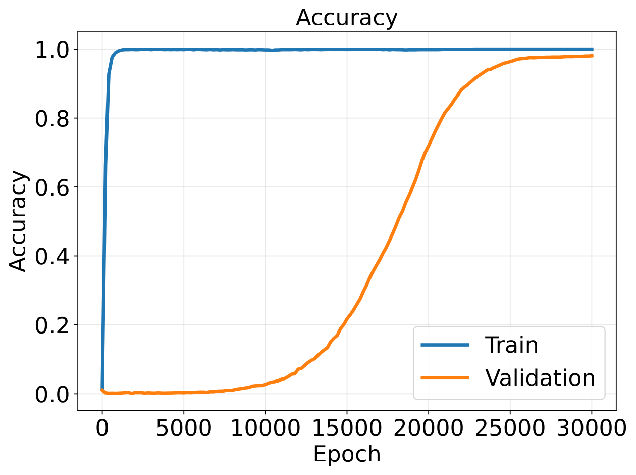
Grokking occurs when a neural network sharply transitions from a memorized to a generalized state. It first reaches almost perfect training accuracy while its validation accuracy remains near chance.¹1. Throughout this post, “validation” refers to the held-out part of the training distribution. After many more updates, validation accuracy rises abruptly, even though the training data has not changed. The network appears to move from memorizing examples to learning the “rule” behind them. We study what changes inside the network during that delay.

1. Grokking and Modular Addition

We start by reviewing some of the background and describing the setup to arrive at the phenomenon of grokking.

1.1 Short Literature Review

Power et al. first observed grokking as delayed generalization on small algorithmic datasets. Their experiments showed that long training and regularization can produce a sudden transition in validation accuracy well after overfitting. Later work aimed at describing the mechanistic and theoretical origin of the transition.

Nanda et al. mechanistically investigated modular-addition transformers. They found a Fourier circuit that forms gradually beneath the sharp accuracy transition. Memorizing components dominate first, Fourier components grow later, and cleanup removes the remaining memorizing structure.

The recent work by Xu et al. analyzes a simple enough model to be solved exactly. Ridge regression can be exactly solved on an over-parameterized linear model, trained by gradient descent with weight decay. They bound the generalization time in terms of the training hyperparameters. Their model traces feature learning back to an ill conditioned initialization through a fixed set of features.

Other studies expanded the phase diagram under different hyperparameters. Doshi et al. separated comprehension, grokking, memorization, confusion, and forgetting on corrupted arithmetic data. We aim to add to the growing literature by providing an analytical perspective on the learning dynamics in ReLU MLPs.

1.2 Setup

Effective theories of Grokking can be reached by restriction of the model class. Liu et al. work with a constrained model, where an embedding forces a group operation. The symbols $a$ and $b$ are mapped to trainable embedding vectors, the two vectors are added, and a small decoder network reads the sum. One is then able to write down an effective theory for the embedding vectors $E_i$, which replicates the empirical experiments of the training dynamics of the neural network. We take a similar approach by assuming a homogeneous neural network:

where $\theta$ are the stacked weights of the neural network $f_\theta$ and $D$ is the degree of homogeneity. This assumption is satisfied by for example ReLU MLPs. This restriction allows us to analyze the gradient flow dynamics on the level of individual samples and integrating out weights directly.

1.3 Decomposition of Modular Addition

We achieve Grokking through modulo addition. Our learning task is therefore addition modulo a prime $p$:

The inputs and outputs are one-hot encoded. We also one-hot encode the output numeral $c$. Modulo addition is periodic with even frequencies $\frac{k}{p}$. The natural basis on this cyclic space consists of the characters

One can therefore decompose the target into a linear combination of fourier features:

Only products with the same frequency $k$ on both input sectors $a,b$ appear. We can therefore hypothesize, that learning Fourier features with the same frequency in both $a,b$ will be useful for generalization. A network encoding these features in its last layer, can linearly solve for the generalization rule.

1.4 Experimental Setup and Gradient-Flow Dynamics

We use $p=23$ producing 529 input pairs, a bias free, one hidden-layer ReLU network of width $256$, trained with full-batch gradient descent on Regression Loss and Weight Decay. We stack the two one-hot encodings of the inputs $a$ and $b$ as an input and directly regress on the one-hot encoded label $c$. We structure the train-validation split by drawing from

where we draw 16 values from $\mathbb Z_p$. ²2. This split is designed to preserve circulant matrices, but is not necessarily needed for the empirical analysis. To describe the learning dynamics without carrying an output-class index through every equation, first consider one scalar output $f_\theta(x)$. We define its prediction error by the residual:

Together with Weight Decay, the loss objective becomes:

Our equations of motion are given by gradient descent.

The first term is given by the regression objective. It is described by the empirical Neural Tangent Kernel, $K(x,x’)=\nabla_\theta f_\theta(x)\cdot\nabla_\theta f_\theta(x’)$. The second term pulls every weight toward the origin. For a homogeneous neural network this amounts to reducing the output magnitude. This relation allows us to rewrite the equations of motion on the level of function space:

For a degree-$D$ homogeneous network, Euler’s relation gives $\nabla_\theta f_\theta(x)\cdot\theta=D,f_\theta(x)$ and so the equations integrate out the weight contributions. This is remarkable, as it allows us to ignore weights in our analysis, which are the crux of most interpretability works. This allows us to directly interpret Gradient Flow as a dynamical system between samples in the training and validation distribution. We are interested in the deviation of our neural network from the labels and therefore investigate the evolution of the residuals of each sample $\sigma^\mu$.

With $D=2$ for the ReLU one-hidden layer neural network, the equations become:

Weight Decay forces a relaxation of the prediction. For samples with $y^\mu=0$, this amounts to an increase in prediction accuracy. This is why we see an increase in the relaxation rate $(\Lambda_\alpha+2\lambda_W)$. For samples with $y^\mu\neq 0$, Weight Decay induces an irreducible loss, which is supported by the source $-2\lambda_W y^\mu$ in the equations of motion. For a constant Kernel $K$, the dynamics reach the kernel ridge regression solution:

Weight decay therefore leaves a residual behind, of size proportional to $\lambda_W$. One can also observe, that the only way to reduce the regression loss of this solution is to increase the alignment of $K$ with the label space $y^\mu$, while kernel modes independent of the target do not contribute. We therefore conclude, that for homogeneous neural networks, the dynamics are mainly driven by the empirical Neural Tangent Kernel and will in the following analyze the learning dynamics from this perspective.

2. Generalization with Tangent Features

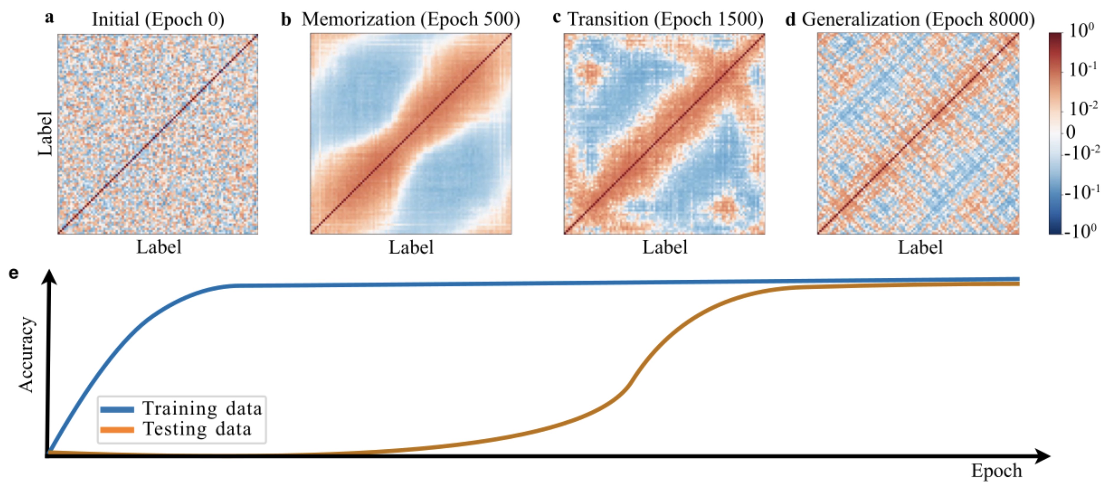
We first inspect the NTK $K^{\mu\nu}$ throughout one grokking run. At initialization it has little visible organization. During memorization it develops broad local structure. Near the validation-accuracy transition, repeated diagonal bands appear and then sharpen into a fine grained periodic pattern. This first observation prompted the empirical and theoretical investigation of the NTK presented here.

2.1 Investigation of the Eigenspectrum

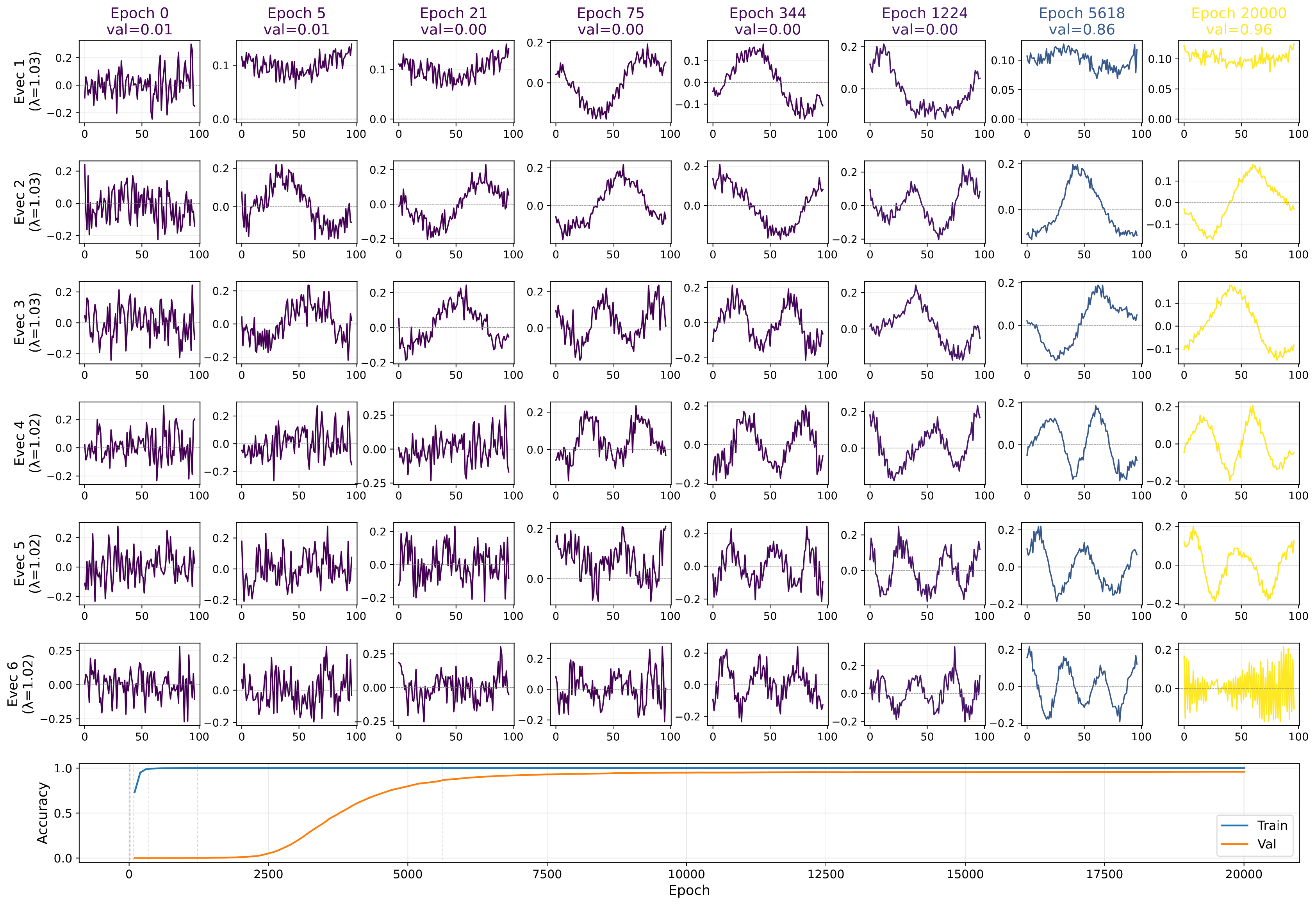
We want to understand, how this fine structure relates to generalization. To this end, we investigate the Kernel Eigenspectrum and how it relates to the label space. We plot the components of the eigenvectors with the 6 highest eigenvalues, which dominate the residual dynamics. Before generalization the eigenvectors are noisy. At the generalization boundary, we observe the emergence of standing waves in label space. These correspond directly to the characters with same frequency in both $a,b$ Fourier Sectors as described in section 1.3. As training continues, the highest eigenvalue eigenvectors emerge as standing waves over the modulo labels. This makes sense as it allows the neural network to discover the data generating rule by a linear combination of these features, which is how a homogeneous neural network produces its prediction. These standing waves are aligned with the target and therefore reduce the loss reached in the ridge regression equilibrium.

2.2 Evolution of Kernel Eigenmodes and the Neural Tangent Hierarchy

We now understand what structure emerges during the generalization transition in grokking modular arithmetic. However, the theoretical explanation for the delayed generalization through feature learning is still unclear. We investigate the evolution of the NTK $K$ during Gradient Flow. For this we employ the Neural Tangent Hierarchy of Huang and Yau. The evolution of the NTK produces a second object $K^{(2)}(x,x’;z)$, which then produces a fourth and onwards. The Neural Tangent Kernel and all higher order modes are again homogeneous functions allowing the integration of the Weight Decay terms. The coupled equations become:

In the NTK initialization, the evolution of $K^{(2)}$ is suppressed by orders of the width $m$ with $K$ becoming constant in the infinite width limit. This gives us intuition that for finite width, we might be able to close the Neural Tangent Hierarchy and treat $K^{(2)}$ as constant. The $\boldsymbol\sigma$ term changes different kernel entries according to the current residuals. The weight Decay term instead exponentially decays every entry of $K$ directly. The growth of the NTK is then directly coupled to the remaining prediction residual.

We now decompose into NTK Fourier modes and write the same equations for each Fourier direction ³3. At initialization, one can explicitly compute the infinite width Neural Tangent Kernel, which then only depends on differences of inputs. By the convolution theorem, this Kernel is then diagonal in Fourier Space, which allows us to approximately track the evolution of each of the Fourier modes independently over time. Additionally, each Fourier mode (besides constant sectors) has equal weight at initialization with one-hot encoded inputs and outputs. This leads to the memorization solution at the start of the training, where all modes are used equally and allows us to focus on a single mode analysis, which will hold for all leaving an effective diagonal $K^{(2)}$. . Let $\Lambda$ be the eigenvalue of $K$ along a chosen Fourier vector $(a,b)$, and let $\sigma$ and $y$ be the residual and target components along that vector. Applying $K^{(2)}$ to the same vector on its first two indices and to the mode residual on its third leaves a scalar coefficient, which we call $a$. We now apply the Neural Tangent Hierarchy and set $a$ approximately as a positive constant. This closure allows us to analytically investigate the dynamics. ⁴4. Further empirical analysis has shown that $a$ evolves quite a bit, but qualitatively the results of the constant $a$ closure fit quite well. Expansions of $a$ in $K$ also seem promising. Using quadratic activation functions should also yield an analytical closure without approximations. Our canonical mode-wise equations become

Structurally these equations are very simple! Surprisingly, they capture most of the qualitative observations during Grokking. Residuals $\sigma$ relax exponentially fast onto the ridge regression solution on the time scale of single Gradient Descent steps $t$. The evolution of features is driven by the remaining residual, which is induced by Weight Decay. This leads to a slow time scale $\tau = \lambda_W\cdot t$. Feature learning is driven through alignment with residuals, while weight decay removes eigenvalues through exponential decay $-2\lambda_W\Lambda$. A target aligned eigenvalue carries a persistent residual source. An unsupported mode does not and decays. We can move from first order differential equations to a closed second order equation for the eigenvalues $\Lambda$. ⁵5. In Dynamical Systems, one usually does the opposite trick and moves from a single variable to a two dimensional phase space. However, in this case, we will describe the second order dynamics from the perspective of a potential to reach some insights and then go back to a Hamiltonian Formulation.

Second Order Equation for Eigenmodes

We can eliminate $\sigma$ exactly. Differentiate the equation for $\Lambda$, use the equation for $\dot\sigma$, and replace $\sigma$ by $-(\dot\Lambda+2\lambda_W\Lambda)/a$. The result closes entirely on the eigenvalue:

This has the form of a damped Newton equation,

For physical eigenvalues $\Lambda\geq0$, the friction $\Gamma$ is positive. The mechanical energy $\mathcal H=\dot\Lambda^2/2+V(\Lambda)$ therefore decreases as

Every Fourier mode follows this same potential equation. What differs is the source $a y$. A mode absent from the target has $a y=0$, so its potential has its physical minimum at $\Lambda=0$ and Weight Decay removes it. A target aligned mode has $a y>0$, which tilts the potential toward a positive minimum. Starting from similar eigenvalues, aligned and non aligned modes therefore move toward different endpoints. This also explains the abrupt transition from a memorized to a generalized state. As all eigenvalues start at the same initial condition, they all cross a critical boundary $\Lambda_{grok}$ at the same time, when they become useful for the ridge regression fit and the network suddenly generalizes. Grokking is then just a phenomenon of an ill-conditioned initialization, which evolves on a timescale of $\lambda_W\cdot t$ to the well-conditioned solution.

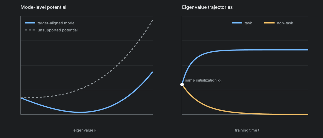
The second order equation retains the full two-state dynamics. It is useful for visualizing why modes separate. To calculate the actual grokking time, we now return to the two first order equations and use the observed fact that their timescales are different.

Effective Adiabatic Approximation of Grokking

The residual relaxes faster than the eigenvalue changes. ⁶6. This assumption is partly given empirically, but qualitatively the results fit the observations very well. Setting $\dot\sigma\simeq0$ gives

Substituting this value as a time scale separation into the second equation leaves one slow equation:

The remaining residual pushes a target mode upward, while weight decay pulls every mode downward. The positive fixed point is

2.3 Theory and the Empirical Phase Diagram

The equations above use continuous gradient-flow time $t$. A discrete run with learning rate $\eta$ and $s$ updates corresponds to $t=\eta s$. After including Weight Decay, the slow clock is $\tau=\eta\lambda_W s$. For the remainder of this section, we absorb the fixed target projection into the mode coupling and write $a$ for the product $a y$. For a budget of $T$ updates, the smallest learning rate for which $\Lambda(\eta\lambda_W T)$ reaches the threshold $\Lambda_{\rm grok}$ from initialization $\Lambda_0$ obeys

To evaluate the integral, factor its denominator using the two fixed points

The partial fraction decomposition gives

so that

Integration gives the explicit critical learning rate

This expression is finite only while the positive fixed point lies above the grokking threshold. Setting $\Lambda_+=\Lambda_{\rm grok}$ gives the vertical feature-learning boundary

These equations predict a U shaped boundary in the $(\lambda_W,\eta)$ plane. Its two limits have the forms:

Below the U-curve, training fits the observed examples but feature learning is too slow, so the network memorizes. Above the curve and below $\lambda_{\rm feature}$, the task modes cross $\Lambda_{\rm grok}$ within $T$ steps and the network groks. For $\lambda_W\geq\lambda_{\rm feature}$, no learning rate can raise the fixed point above the task threshold in the continuous theory, so the network remains in the memorizing or high-decay region.

A second, nearly vertical boundary comes from the fast kernel ridge regression fit. If a training mode with eigenvalue $\Lambda_{\rm fit}$ must retain a fraction $g_{\min}$ of its target, then

Beyond $\lambda_{\rm fit}$, Weight Decay is too big even for the training fit. Between $\lambda_{\rm feature}$ and $\lambda_{\rm fit}$, the network can fit without sustaining the task modes. This is where memorization reaches a partly resolved forgetting/no-fitting region. Finally, discrete gradient descent requires the learning rate to remain below the edge of stability, approximately $\eta_{\rm cut}\simeq2/\alpha_{\max}$ for the largest effective curvature $\alpha_{\max}$. This adds the horizontal upper edge missing for approximating Gradient Flow.

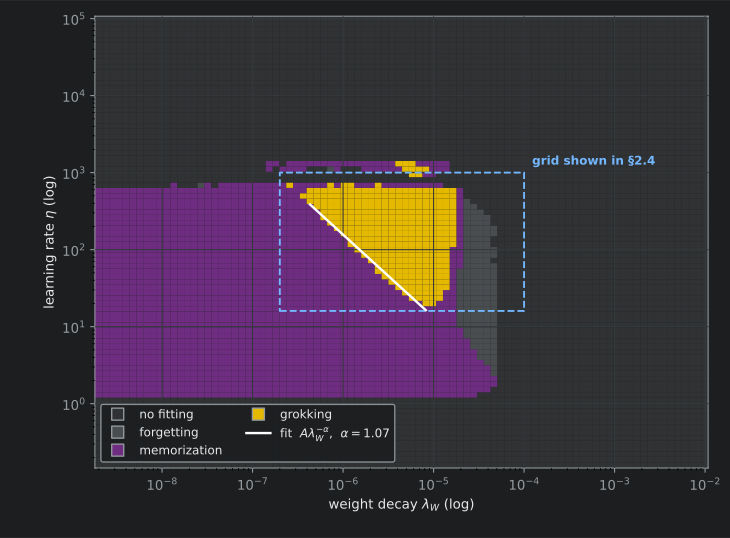
We test this against a single $p=23$ empirical sweep. We cover an $84\times90$ grid in $(\eta,\lambda_W)$, with the learning rate running from $16$ to $1000$ and Weight Decay from $2\times10^{-7}$ to $10^{-4}$, both logarithmically spaced to observe the predicted linear Grokking boundary.⁷7. The comically large learning rates originate from averaging of the full batch regression loss producing small values. This gives us 7,560 runs of $T=24,000$ full-batch updates each.

Figure 5 shows the phase diagram and its 3.5 phases. In the grokking phase, both training and validation accuracy exceed 90%. In memorization, only training accuracy does. At larger Weight Decay, some runs fit and then forget. The neighboring no-fitting label means that no fit was recorded. We therefore treat forgetting and no fitting as one partly resolved region rather than two firmly separated phases. We find remarkable agreement between our linear adiabatic Grokking boundary and the empirically observed phase diagram. Interestingly, there appears to be a small grokking island at very high values of learning rates, which has interesting training curves and should be investigated further. Both the u-shape and the linear grokking boundary fit very well. Larger time horizons would extend the grokking boundary further into the lower left corner of phase space. For a larger sweep, please view the Appendix.

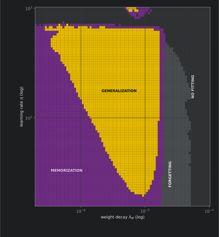
Figure 5. Predicted and observed phase structure, compared qualitatively. Yellow represents grokking, purple memorization, and the gray high-decay region denotes forgetting/no fitting. The empirical panel uses a lighter gray to distinguish observed forgetting from no fitting. The experimental panel contains the complete fixed split grid. Experimental Setup B.

2.4 Inducing Grokking Through Feature Transfer

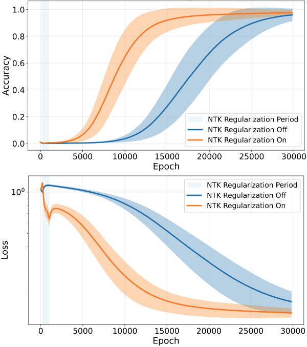
We want to test our theory by inducing the right Kernel structure from the start of the training and induce Grokking. To do this, we train a source network until it generalizes and record the label averaged and projected onto the true label space NTK, $\bar{K}_{\rm gen}$. This matrix is transferred to a fresh network through the temporary regularization

This encourages the new network to begin with stronger interactions along the target aligned directions. We extract the generalized NTK from a two-hidden-layer ReLU network with width 256. As a target we use a three-hidden layer network of width 128 trained on a different training-validation split. We activate the penalty only for the first 800 epochs to imitate initialization.

Across 50 different seeds, the biased networks generalize earlier. Their validation loss drops during the short regularization period and remains below the baseline after the penalty is removed. Transferring $\bar K_{\rm gen}$ therefore supports the theoretical analysis.

3. Conclusion and Takeaways

We conclude that Grokking in homogeneous neural networks is sparked via a regularizing pressure of Weight Decay and is a gradual process where the Neural Tangent Kernel aligns with the training labels over time. In our experimental setup the abrupt transition from a memorized to a generalized state is induced via a conjoint movement of all features related to generalization yielding a sigmoid like transition. This depends on the one-hot encoding of our inputs, as it forces the same initial condition on all Fourier Modes with no bias to larger or smaller wave lengths. This is in contrast to other tasks (Image classification with CNNs), where inductive bias is helpful for generalization. Our analysis is also limited to algorithmic datasets. Grokking has however been observed in more general settings, where it might have a different origin. Our theoretical analysis is however independent of the exact group structure and could be extended to a more general theory of feature learning, where the canonical basis of the underlying task is less well known.

To summarize in three points:

• Memorization and generalization use different NTK spectra. A broad initial spectrum can fit observed examples, while the modular rule requires stronger equal-frequency Fourier modes.
• Grokking Through Feature Learning. Training accuracy saturates and Weight Decay induces a time scale on the order of $\lambda_W\cdot t$, under which the Tangent Features evolve. In these networks, Grokking occurs through actual feature learning.
• We can enforce an inductive bias through regularization Temporarily steering a new network toward a generalized NTK makes it generalize sooner.

Compute

The phase sweep ran on NVIDIA A40 GPU slices.

References

1. Alethea Power et al. Grokking: Generalization Beyond Overfitting on Small Algorithmic Datasets, 2022.
2. Mingyue Xu, Gal Vardi, and Itay Safran. To Grok Grokking: Provable Grokking in Ridge Regression, ICML 2026.
3. Neel Nanda et al. Progress Measures for Grokking via Mechanistic Interpretability, 2023.
4. Darshil Doshi et al. To Grok or Not to Grok: Disentangling Generalization and Memorization on Corrupted Algorithmic Datasets, 2024.
5. Ziming Liu et al. Towards Understanding Grokking: An Effective Theory of Representation Learning, 2022.
6. Arthur Jacot, Franck Gabriel, and Clément Hongler. Neural Tangent Kernel: Convergence and Generalization in Neural Networks, 2018.
7. Jiaoyang Huang and Horng-Tzer Yau. Dynamics of Deep Neural Networks and Neural Tangent Hierarchy, 2020.

Cite This Work

Lenz Pracher, Pascal de Jong, Oskar Liesaus, Alan Jeffares, and Steffen Rulands. “A Spectral Theory of Grokking.” 2026.

@misc{pracher2026grokking,
  title  = {A Spectral Theory of Grokking},
  author = {Pracher, Lenz and de Jong, Pascal and Liesaus, Oskar and Jeffares, Alan and Rulands, Steffen},
  year   = {2026},
  url    = {https://lenzpracher.github.io/projects/grokking/}
}

Comments

Appendix

A.1 Experimental Setups

Two different models appear in this post. We used preliminary experiments (Setup A) that motivated the theory, which then promoted a simplified setup (Setup B). The phase maps use the simplified Setup B, while the rest of the figures used Setup A.

Setup A — preliminary experiments. Modular addition on $\mathbb Z_p$ with $p=97$. The symbols $a$ and $b$ are one-hot encoded and concatenated, $(e_a\oplus e_b)\in\mathbb R^{2p}$, and the target is the one-hot encoding of $f(a,b)$ in $\mathbb R^{p}$. Commutativity leaves $p(p+1)/2$ unique mappings, which make up the training and validation set. The training and validation sets are formed by drawing a fraction $r=0.5$ of those unique mappings. The model used is a bias-free ReLU MLP with two hidden layers of width 256 under HeNormal initialization, trained by full-batch gradient descent with Weight Decay for 20,000 epochs. The loss used was a weighted squared error in which the true label coordinate carries weight $d_O-1$ and each of the $d_O-1$ off-label coordinates carries weight 1, so that true and off-label terms contribute equal total mass. The kernel shown is the label-averaged projected NTK onto the true labels. The label averaging works by averaging the NTK samples, which have the same label. For example $(a_1,b_1) = (2,3)$ would be averaged with $(a_2,b_2)=(4,1)$. This was done to extract the label wise structure. The transfer experiment trains a teacher of two hidden layers of width 256 to generalization, then adds $\lambda_{\rm focus}\lVert\bar G_S-\bar G_T\rVert_F$ to the loss of a student with three hidden layers of width 128 for the first 800 epochs, with a different split, a different initialization distribution and different hyperparameters, repeated over 50 runs.

Setup B — simplified model. Modular addition on $\mathbb Z_{23}$, with both orders of every pair retained, so the kernel is evaluated on all $23^2=529$ input pairs. The symbols $a$ and $b$ are one-hot encoded and the target is the one-hot encoding from the sum, where the input is concatenated. The model used is a bias-free ReLU network with a single hidden layer of width 256, which makes it degree two homogeneous, trained by full-batch gradient descent on the plain regular squared loss with L2 Weight Decay for 24,000 updates. The training and validation split is structured by input differences. 16 residues $D\subset\mathbb Z_{23}$ are drawn once and training uses ${(a,b):a-b\bmod 23\in D}$, giving 368 training and 161 held-out pairs at $r=16/23$. One fixed split and one model seed are used at every grid point.

The two differ mostly through choice of the loss. We found that regular regression loss also works, while Setup A chose a loss to imitate cross entropy loss. The train and validation split is also simplified to be compatible with the Fourier basis.

A.2 The Expanded Phase Map